Python Pitfalls

source 1, source 2

#1: Misusing expressions as defaults for function arguments

Python allows you to specify that a function argument is optional by providing a default value for it. While this is a great feature of the language, it can lead to some confusion when the default value is mutable. For example, consider this Python function definition:

>>> def foo(bar=[]):        # bar is optional and defaults to [] if not specified
...    bar.append("baz")    # but this line could be problematic, as we'll see...
...    return bar

A common mistake is to think that the optional argument will be set to the specified default expression each time the function is called without supplying a value for the optional argument. In the above code, for example, one might expect that calling foo() repeatedly (i.e., without specifying a bar argument) would always return 'baz', since the assumption would be that each time foo() is called (without a bar argument specified) bar is set to [] (i.e., a new empty list).
But let’s look at what actually happens when you do this:

>>> foo()
["baz"]
>>> foo()
["baz", "baz"]
>>> foo()
["baz", "baz", "baz"]

Huh? Why did it keep appending the default value of "baz" to an existing list each time foo() was called, rather than creating a new list each time?
The answer is that the default value for a function argument is only evaluated once, at the time that the function is defined. Thus, the bar argument is initialized to its default (i.e., an empty list) only when foo() is first defined, but then calls to foo() (i.e., without a bar argument specified) will continue to use the same list to which bar was originally initialized.
FYI, a common workaround for this is as follows:

>>> def foo(bar=None):
...    if bar is None:  # or if not bar:
...        bar = []
...    bar.append("baz")
...    return bar
...
>>> foo()
["baz"]
>>> foo()
["baz"]
>>> foo()
["baz"]

#2: Using class variables incorrectly

Consider the following example:

>>> class A(object):
...     x = 1
...
>>> class B(A):
...     pass
...
>>> class C(A):
...     pass
...
>>> print A.x, B.x, C.x
1 1 1

Makes sense.

>>> B.x = 2
>>> print A.x, B.x, C.x
1 2 1

Yup, again as expected.

>>> A.x = 3
>>> print A.x, B.x, C.x
3 2 3

What the $%#!&?? We only changed A.x. Why did C.x change too?
In Python, class variables are internally handled as dictionaries and follow what is often referred to as Method Resolution Order (MRO). So in the above code, since the attribute x is not found in class C, it will be looked up in its base classes (only A in the above example, although Python supports multiple inheritance). In other words, C doesn’t have its own x property, independent of A. Thus, references to C.x are in fact references to A.x.

#3: Specifying parameters incorrectly for an exception block

Suppose you have the following code:

>>> try:
...     l = ["a", "b"]
...     int(l[2])
... except ValueError, IndexError:  # To catch both exceptions, right?
...     pass
...
Traceback (most recent call last):
  File "", line 3, in 
IndexError: list index out of range

The problem here is that the except statement does not take a list of exceptions specified in this manner. Rather, In Python 2.x, the syntax except Exception, e is used to bind the exception to the optional second parameter specified (in this case e), in order to make it available for further inspection. As a result, in the above code, the IndexError exception is not being caught by the except statement; rather, the exception instead ends up being bound to a parameter named IndexError.
The proper way to catch multiple exceptions in an except statement is to specify the first parameter as a tuple containing all exceptions to be caught. Also, for maximum portability, use the as keyword, since that syntax is supported by both Python 2 and Python 3:

>>> try:
...     l = ["a", "b"]
...     int(l[2])
... except (ValueError, IndexError) as e:  
...     pass
...
>>>

#4: Misunderstanding Python scope rules

Python scope resolution is based on what is known as the LEGB rule, which is shorthand for Local, Enclosing, Global, Built-in. Seems straightforward enough, right? Well, actually, there are some subtleties to the way this works in Python. Consider the following:

>>> x = 10
>>> def foo():
...     x += 1
...     print x
...
>>> foo()
Traceback (most recent call last):
  File "", line 1, in 
  File "", line 2, in foo
UnboundLocalError: local variable 'x' referenced before assignment

What’s the problem?
The above error occurs because, when you make an assignment to a variable in a scope, that variable is automatically considered by Python to be local to that scope and shadows any similarly named variable in any outer scope.
Many are thereby surprised to get an UnboundLocalError in previously working code when it is modified by adding an assignment statement somewhere in the body of a function. (You can read more about this here.)
It is particularly common for this to trip up developers when using lists. Consider the following example:

>>> lst = [1, 2, 3]
>>> def foo1():
...     lst.append(5)   # This works ok...
...
>>> foo1()
>>> lst
[1, 2, 3, 5]

>>> lst = [1, 2, 3]
>>> def foo2():
...     lst += [5]      # ... but this bombs!
...
>>> foo2()
Traceback (most recent call last):
  File "", line 1, in 
  File "", line 2, in foo
UnboundLocalError: local variable 'lst' referenced before assignment

Huh? Why did foo2 bomb while foo1 ran fine?
The answer is the same as in the prior example, but is admittedly more subtle. foo1 is not making an assignment to lst, whereas foo2 is. Remembering that lst += [5] is really just shorthand for lst = lst + [5], we see that we are attempting to assign a value to lst (therefore presumed by Python to be in the local scope). However, the value we are looking to assign to lst is based on lst itself (again, now presumed to be in the local scope), which has not yet been defined. Boom.

#5: Modifying a list while iterating over it 

The problem with the following code should be fairly obvious:

>>> odd = lambda x : bool(x % 2)
>>> numbers = [n for n in range(10)]
>>> for i in range(len(numbers)):
...     if odd(numbers[i]):
...         del numbers[i]  # BAD: Deleting item from a list while iterating over it
...
Traceback (most recent call last):
     File "", line 2, in 
IndexError: list index out of range

Deleting an item from a list or array while iterating over it is a faux pas well known to any experienced software developer. But while the example above may be fairly obvious, even advanced developers can be unintentionally bitten by this in code that is much more complex.
Fortunately, Python incorporates a number of elegant programming paradigms which, when used properly, can result in significantly simplified and streamlined code. A side benefit of this is that simpler code is less likely to be bitten by the accidental-deletion-of-a-list-item-while-iterating-over-it bug. One such paradigm is that of list comprehensions. Moreover, list comprehensions are particularly useful for avoiding this specific problem, as shown by this alternate implementation of the above code which works perfectly:

>>> odd = lambda x : bool(x % 2)
>>> numbers = [n for n in range(10)]
>>> numbers[:] = [n for n in numbers if not odd(n)]  # ahh, the beauty of it all
>>> numbers
[0, 2, 4, 6, 8]

#6: Confusing how Python binds variables in closures

Considering the following example:

>>> def create_multipliers():
...     return [lambda x : i * x for i in range(5)]
>>> for multiplier in create_multipliers():
...     print multiplier(2)
...

You might expect the following output:

0
2
4
6
8

But you actually get:

8
8
8
8
8

Surprise!
This happens due to Python’s late binding behavior which says that the values of variables used in closures are looked up at the time the inner function is called. So in the above code, whenever any of the returned functions are called, the value of i is looked up in the surrounding scope at the time it is called (and by then, the loop has completed, so i has already been assigned its final value of 4).
The solution to this is a bit of a hack:

>>> def create_multipliers():
...     return [lambda x, i=i : i * x for i in range(5)]
...
>>> for multiplier in create_multipliers():
...     print multiplier(2)
...
0
2
4
6
8

Voilà! We are taking advantage of default arguments here to generate anonymous functions in order to achieve the desired behavior. Some would call this elegant. Some would call it subtle. Some hate it. But if you’re a Python developer, it’s important to understand in any case.

#7: Creating circular module dependencies

Let’s say you have two files, a.py and b.py, each of which imports the other, as follows:
In a.py:

import b

def f():
    return b.x
 
print f()

And in b.py:

import a

x = 1

def g():
    print a.f()

First, let’s try importing a.py:

>>> import a
1

Worked just fine. Perhaps that surprises you. After all, we do have a circular import here which presumably should be a problem, shouldn’t it?
The answer is that the mere presence of a circular import is not in and of itself a problem in Python. If a module has already been imported, Python is smart enough not to try to re-import it. However, depending on the point at which each module is attempting to access functions or variables defined in the other, you may indeed run into problems.
So returning to our example, when we imported a.py, it had no problem importing b.py, since b.py does not require anything from a.py to be defined at the time it is imported. The only reference in b.py to a is the call to a.f(). But that call is in g() and nothing in a.py or b.py invokes g(). So life is good.
But what happens if we attempt to import b.py (without having previously imported a.py, that is):

>>> import b
Traceback (most recent call last):
     File "", line 1, in <module>
     File "b.py", line 1, in <module>
    import a
     File "a.py", line 6, in <module>
 print f()
     File "a.py", line 4, in f
 return b.x
AttributeError: 'module' object has no attribute 'x'

Uh-oh. That’s not good! The problem here is that, in the process of importing b.py, it attempts to import a.py, which in turn calls f(), which attempts to access b.x. But b.x has not yet been defined. Hence the AttributeError exception.
At least one solution to this is quite trivial. Simply modify b.py to import a.py within g():

x = 1

def g():
    import a # This will be evaluated only when g() is called
    print a.f()

No when we import it, everything is fine:

>>> import b
>>> b.g()
1 # Printed a first time since module 'a' calls 'print f()' at the end
1 # Printed a second time, this one is our call to 'g'

#8: Name clashing with Python Standard Library modules

One of the beauties of Python is the wealth of library modules that it comes with “out of the box”. But as a result, if you’re not consciously avoiding it, it’s not that difficult to run into a name clash between the name of one of your modules and a module with the same name in the standard library that ships with Python (for example, you might have a module named email.py in your code, which would be in conflict with the standard library module of the same name).
This can lead to gnarly problems, such as importing another library which in turns tries to import the Python Standard Library version of a module but, since you have a module with the same name, the other package mistakenly imports your version instead of the one within the Python Standard Library. This is where bad stuff happens.
Care should therefore be exercised to avoid using the same names as those in the Python Standard Library modules. It’s way easier for you to change the name of a module within your package than it is to file a Python Enhancement Proposal (PEP) to request a name change upstream and to try and get that approved.

#9: Failing to address differences between Python 2 and Python 3

Consider the following file foo.py:

import sys

def bar(i):
    if i == 1:
        raise KeyError(1)
    if i == 2:
        raise ValueError(2)

def bad():
    e = None
    try:
        bar(int(sys.argv[1]))
    except KeyError as e:
        print('key error')
    except ValueError as e:
        print('value error')
    print(e)

bad()

On Python 2, this runs fine:

$ python foo.py 1
key error
1
$ python foo.py 2
value error
2

But now let’s give it a whirl on Python 3:

$ python3 foo.py 1
key error
Traceback (most recent call last):
  File "foo.py", line 19, in 
    bad()
  File "foo.py", line 17, in bad
    print(e)
UnboundLocalError: local variable 'e' referenced before assignment

What has just happened here? The “problem” is that, in Python 3, the exception object is not accessible beyond the scope of the except block. (The reason for this is that, otherwise, it would keep a reference cycle with the stack frame in memory until the garbage collector runs and purges the references from memory. More technical detail about this is available here).
One way to avoid this issue is to maintain a reference to the exception object outside the scope of the except block so that it remains accessible. Here’s a version of the previous example that uses this technique, thereby yielding code that is both Python 2 and Python 3 friendly:

import sys

def bar(i):
    if i == 1:
        raise KeyError(1)
    if i == 2:
        raise ValueError(2)

def good():
    exception = None
    try:
        bar(int(sys.argv[1]))
    except KeyError as e:
        exception = e
        print('key error')
    except ValueError as e:
        exception = e
        print('value error')
    print(exception)

good()

Running this on Py3k:

$ python3 foo.py 1
key error
1
$ python3 foo.py 2
value error
2

Yippee!

#10: Misusing the __del__ method

Let’s say you had this in a file called mod.py:

import foo

class Bar(object):
        ...
    def __del__(self):
        foo.cleanup(self.myhandle)

And you then tried to do this from another_mod.py:

import mod
mybar = mod.Bar()

You’d get an ugly AttributeError exception.
Why? Because, as reported here, when the interpreter shuts down, the module’s global variables are all set to None. As a result, in the above example, at the point that __del__ is invoked, the name foo has already been set to None.
A solution would be to use atexit.register() instead. That way, when your program is finished executing (when exiting normally, that is), your registered handlers are kicked off before the interpreter is shut down.
With that understanding, a fix for the above mod.py code might then look something like this:

import foo
import atexit

def cleanup(handle):
    foo.cleanup(handle)


class Bar(object):
    def __init__(self):
        ...
        atexit.register(cleanup, self.myhandle)

This implementation provides a clean and reliable way of calling any needed cleanup functionality upon normal program termination. Obviously, it’s up to foo.cleanup to decide what to do with the object bound to the name self.myhandle, but you get the idea. But while were at it..

#11: __del__ Can't be Trusted

The mere existence of this method makes objects that are part of a reference cycle uncollectable by Python's garbage collector and could lead to memory leaks.
Use a weakref.ref object with a callback to run code when an object is being removed instead.
See also Python gc module documentation

#12: Using os.system or os.popen instead of subprocess

Starting with the non-controversial: Anything that has been marked deprecated should be avoided. The deprecation warning should have instructions with safe alternatives you can use.
Some of the most frequent offenders are parts of the language that make it difficult to safely call other programs:

os.system()

os.popen()

import commands

We have the excellent subprocess module for these now, use it.

#13: Not using duck typing

Explicitly checking the type of a parameter passed to a function breaks the expected duck-typing convention of Python. Common type checking includes:

isinstance(x, X)

type(x) == X

With type() being the worse of the two.
If you must have different behaviour for different types of objects passed, try treating the object as the first data type you expect, and catching the failure if that type wasn't that type, and then try the second. This allows users to create objects that are close enough to the types you expect and still use your code.
See also isinstance() considered harmful.

#14: Using pickle to serialize data

import pickle # or cPickle

Objects serialized with pickle are tied to their implementations in the code at that time. Restoring an object after an underlying class has changed will lead to undefined behaviour. Unserializing pickled data from an untrusted source can lead to remote exploits. The pickled data itself is opaque binary that can't be easily edited or reviewed.
This leaves only one place where pickle makes sense -- short lived data being passed between processes, just like what the multiprocessing module does.
Anywhere else use a different format. Use a database or use JSON with a well-defined structure. Both are restricted to simple data types and are easily verified or updated outside of your Python script. See also Alex Gaynor's presentation on pickle.

#15: Misusing demonstration modules

Many people are drawn to these modules because they are part of Python's standard library. Some people even try to do serious work with them.

import asyncore

import asynchat

import SimpleHTTPServer

The former resembles a reasonable asynchronous library, until you find out there are no timers. At all. Use Twisted or Tornado instead.
The latter makes for a neat demo by letting giving you a web server in your pocket with the one command python -m SimpleHTTPServer. But this code was never intended for production use, and certainly not designed to be run as a public web server. There are plenty of real, hardened web servers out there that will run your python code as a WSGI script. Choose one of them instead.

#16: Using import array

import array

All the flexibility and ease of use of C arrays, now in Python!
If you really really need this you will know. Interfacing with C code in an extension module is one valid reason.
If you're looking for speed, try just using regular python lists with PyPy . Another good choice is NumPy for its much more capable arrays types.

#17: Split Personality

reload(x)

It looks like the code you just changed is there, except the old versions of everything is still there too. Objects created before the reload will still use the code as it was when they were created, leading to situations with interesting effects that are almost impossible to reproduce.
Just re-run your program. If you're debugging at the interactive prompt consider debugging with a small script and python -i instead.

#18: Copy is Almost Reasonable

import copy

The copy module is harmless enough when used on objects that you create and you fully understand. The problem is once you get in the habit of using it, you might be tempted to use it on objects passed to you by code you don't control.
Copying arbitrary objects is troublesome because you will often copy too little or too much. If this object has a reference to an external resource it's unclear what copying that even means. It can also easily lead to subtle bugs introduced into your code by a change outside your code.
If you need a copy of a list or a dict, use list() or dict()``because you can be sure what you will get after they are called.  ``copy(), however might return anything, and that should scare you.

#19: Admit You Always Hated It

if __name__ == '__main__':

This little wart has long been a staple of many python introductions. It lets you treat a python script as a module, or a module as a python script. Clever, sure, but it's better to keep your scripts and modules separate in the first place.
If you treat a module like a script, then something imports the module you're in trouble: now you have two copies of everything in that module.
I have used this trick to make running tests easier, but setuptools already provides a better hook for running tests. For scripts setuptools has an answer too, just give it a name and a function to call, and you're done.
My last criticism is that a single line of python should never be 10 alphanumeric characters and 13 punctuation characters. All those underscores are there as a warning that some special non-obvious language-related thing is going on, and it's not even necessary.
See also setuptools/distribute automatic script creation
and also PEP 366 pointed out by agentultra on HN

#20: Don't Emulate stdlib

It's in standard library, it must be well written, right?
May I present the implementation of namedtuple, which is really handy little class that used properly can significantly improve your code's readability.

def namedtuple(typename, field_names, verbose=False, rename=False):
    # Parse and validate the field names.  Validation serves two purposes,
    # generating informative error messages and preventing template injection attacks.

Wait, what? "preventing template injection attacks"?
This is followed by 27 lines of code that validates field_names. And then:

template = '''class %(typename)s(tuple):
   '%(typename)s(%(argtxt)s)' \n
   __slots__ = () \n
   _fields = %(field_names)r \n
   def __new__(_cls, %(argtxt)s):
       'Create new instance of %(typename)s(%(argtxt)s)'
       return _tuple.__new__(_cls, (%(argtxt)s)) \n
   @classmethod
   def _make(cls, iterable, new=tuple.__new__, len=len):
       'Make a new %(typename)s object from a sequence or iterable'
       result = new(cls, iterable)
       if len(result) != %(numfields)d:
       raise TypeError('Expected %(numfields)d arguments, got %%d' %% len(result))
       return result \n
   def __repr__(self):
       'Return a nicely formatted representation string'
       return '%(typename)s(%(reprtxt)s)' %% self \n
   def _asdict(self):
       'Return a new OrderedDict which maps field names to their values'
       return OrderedDict(zip(self._fields, self)) \n
   __dict__ = property(_asdict) \n
   def _replace(_self, **kwds):
       'Return a new %(typename)s object replacing specified fields with new values'
       result = _self._make(map(kwds.pop, %(field_names)r, _self))
       if kwds:
           raise ValueError('Got unexpected field names: %%r' %% kwds.keys())
       return result \n
   def __getnewargs__(self):
       'Return self as a plain tuple.  Used by copy and pickle.'
       return tuple(self) \n\n''' % locals()

Yes, that's a class definition in a big Python string, filled with variables from locals(). The result is then exec -ed in the right namespace, and some further magic is applied to "fix" copy() and pickle().
I believe this code was meant some sort of warning to people that would contribute code to Python -- something like "We make it look like we know what we're doing, but we're really just nuts" (love ya Raymond)
See also collections.py source code
and also an attempted fix pointed out by ffrinch on reddit

#21: Trying Too Hard

hasattr(obj, 'foo')

hasattr() has always been defined to swallow all exceptions, even ones you might be interested in (such as a KeyboardInterrupt) and turn them into a False return value. This interface just can't be fixed, use getattr() with a sentinel value instead.

#22: Off by One

'hello'.find('H')

str.find() and str.rfind() return -1 on failure. This can lead to some really hard to find bugs when combined with containers like strings that treat -1 as the last element. Use str.index() and str.rindex() instead.

Singleton I love you, but you're bringing me down (repost)

Source (reposted here as it's hard for me to read on that page)

Single(ton), again.

Who among us hasn't smuggled into the break-room to nibble on a Singleton newton? I, like you, drank the Singleton kool-aid. At first Singletons were used appropriately. Then, they were used inappropriately. Then they were used really inappropriately. And somewhere between the appropriate and the inappropriate, you, like me, probably realized that something was amiss. Something was aloof, a little bit off.

Then I, like you, read "Singletons Considered Stupid" by Steve Yeggee:

Why is the Singleton so attractive? I'll be the first to admit: I liked it too. No, scratch that – I loved the Singleton. It felt like an old friend from the moment I laid eyes on it. It was simple and beautiful.

I'll tell you why: it's because the Singleton pattern is a throwback to non-OO programming. It's a lifeline for people who didn't understand a single word that the Gang of Four were trying to say. It's almost exactly the way I programmed back when I didn't know jack squat about OOP. The only significant difference is that instead of having a file with a bunch of global functions in it, I have a file with a CLASS that has a bunch of global functions. No need to worry my little head about how many of them to have, since you only need one! It's OOP made easy.

And my heart was broken.

Then I read article after article about why the Singleton was a piss poor Design Pattern.

I learned that Singletons were actually referred to as something called a "code smell." I didn't know if the smell was good or bad, but we figured it was bad.

I learned that Singletons violated something called the 'Single Responsibility Principle' which states that every class you create should do one thing and one thing only because a Singleton has two distinct responsibilities: policing the instances of itself and providing configuration information.

I learned that Singletons were bad for memory management. If no one uses it for awhile, its just going to sit and twiddle its thumbs.

I learned that the state of the Singleton never goes away. Persistent state is the enemy of unit testing. One of the things that makes unit testing effective is that each test has to be independent of all the others.

I learned that Singleton's are kind of impossible to sub-class because they are static methods and static methods are about "as flexible as granite."

I learned that Singletons are (mostly) used as glorified globals and if you use them in your project, your project becomes almost impossible to unit-test because your "objects can secretly get hold of things which are not declared in their APIs, and, as a result, Singletons make your APIs into pathological liars." Basically, when objects use Singletons they hide their dependencies.

I learned that maybe, just maybe you'll realize somewhere down the line that you actually need TWO instances of the Singleton. Then what, buddy?

So I did what any completely sane Programmer would do. I ripped RIPPED the Singleton Pattern out of GOF and burned the pages while doing a triple hail mary and beat on, boat against the current, swearing never NEVER to use another Singleton for as long as I shall live.

Then, three weeks later, after I sobered up, I realized that all the stuff I learned about why Singletons were the devil incarnate was actually a form of "abstinence only" Design Pattern Education. I knew that I could avoid all the aforementioned problems by simply abstaining completely from using Singletons, but what I didn't know was what happened on the day when I wanted to use a single instance of a class and thought that the Singleton might be the best tool for the job?

Fine. Go ahead, use it.

First, before I answers the question posed above, let me address you. I know you. You're stubborn. You're going to use that Singleton until someone rips it from your cold, dead claws. If this is you, then just read on a little while longer then you can get back to uploading your favorite programming cartoon to stackoverflow.

If you do use Singletons, try to use dependency injection instead of calling getInstance() from the constructor.

Use this:

public MyConstructor(Singleton singleton) {
    this.singleton = singleton;
}

rather than this:

public MyConstructor() {
    this.singleton = Singleton.getInstance();
}

At the very least, using dependency injection allows you to do some unit testing of the class by adhering to good encapsulation principles. Using dependency injection might also stop Misko Hevrey from calling your APIa pathological liar. But probably not.

Check yo-self.

For all the rest of you still reading, before using a Singleton ask yourself, "is a Singleton really the best tool for the job?"

On my quest for the truth I discovered that there are actually very few "acceptable" reasons to use a Singleton.

One reason that tends to come up over and over again on the internets is that of a "logging" class. In this case, a Singleton can be used instead of a single instance of a class because a logging class usually needs to be used over and over again ad nauseam by every class in a project. If every class uses this logging class, dependency injection becomes cumbersome.

Logging is a specific example an "acceptable" Singleton because it doesn't affect the execution of your code. Disable logging, code execution remains the same. Enable it, same same. Misko puts it in the following way inRoot Cause of Singletons, "The information here flows one way: From your application into the logger. Even though loggers are global state, since no information flows from loggers into your application, loggers are acceptable."

I'm sure there are other valid reasons as well. Alex Miller, in "Patterns I Hate", talks of service locators and client side UI's also being possibly "acceptable" choices.

Single Instance Of A Class

In most cases, though, you probably got it wrong when you went to the ole' Singleton toolbox. What you probably wanted was a simple single instance of a class instead of a Singleton. There is absolutely nothing wrong with only wanting a single instance of a class. There are, however, way better ways of managing these instances then a "glorified global".

How do you achieve a Single Configuration Object without using a Singleton? Neal Ford in "The Productive Programmer" suggests "using a plain object plus a factory and delegating the individual responsibilities to each. The factory is responsible for the instance policing and the plain object deals only with configuration information and behavior." By using this technique, your code no longer smells as it now adheres to theSingle Responsibility Principle.

Misko Hevrey (who does testing for google) goes into much greater detail about this technique in his two fantastic blog posts entitled "How to Think About the 'new' Operator with Respect to Unit Testing" and "Where Have All the Singletons Gone?"

The idea is to have either classes with logic or classes with the new operator (factories). When you need a single instance of a logic class, you call on the factory to build that class. Using this technique, all the dependencies are automatically injected into this single instance in proper order and returned to you. All objects of a similar lifetime are grouped into this single factory.

Misko uses the example of building a "House."

class House {
  private final Kitchen kitchen;
  private final Bedroom bedroom;
  private boolean isLocked;
 
   public House(Kitchen kitchen, Bedroom bedroom) {
    this.kitchen = kitchen;
    this.bedroom = bedroom;
  }
 
  private boolean isLocked() {
    return isLocked;
  }
 
  private boolean lock() {
    kitchen.lock();
    isLocked = true;
  }
}

Notice that in the House class, there are no instances of "new." Remember, don't mix new and logic, baby. Like J-Lo and Puffy. All the dependencies needed to build a "House" are injected into the constructor. All the "new" stuff is in the HouseFactory (seen below).

class HouseFactory {
  House build() {
 
     Sink sink = new Sink;
     Dishwasher dishwasher = new Dishwasher;
     Refrigerator refrigerator = new Refrigerator;
     Kitchen kitchen = new Kitchen(sink, dishwasher, refrigerator);
 
 Bed bed = new Bed;
     Dresser dresser = new Dresser;
     Bedroom bedroom = new Bedroom(bed, dresser);
 
 House house = new House(kitchen, bedroom);
 
    return house;
 
  }
}
 
class Main {
  public static void(String...args) {
    House house = new HouseFactory().build();
    house.lock();
  }
}

In the "house" factory, when build() is called, kitchen is created and composed of sink, dishwasher, and refrigerator objects. Bedroom is created and composed of created bed and dresser objects. House is created, composed of kitchen and bedroom objects, then returned to the user.

Using this technique, you can see how easy it will be to achieve a single configuration object without the use of a Singleton. A single instance of HouseBuilder is instantiated in the main and with that comes single instances of house, kitchen, bedroom, sink, dishwasher, refrigerator, bed, and dresser.

Using this technique solves the issue of global state because "there is no global state at all. Every object only has references to what it needs directly! No passing around of objects which are not directly needed by the code. Dependencies are obvious since each object only asks for what it needs."

Using this technique solves the issue of memory management. All classes will be created and used when needed. No more Singletons sitting around and taking up memory while doing nothing at all.

Using this technique you can extend any of the classes you desire. Static methods are nowhere. No-sir.

Using this technique you can Unit-Test without fear of a wolf attack.

Plus, Misko adds:

If an object needs a reference to a new dependency it simply declares it. This change only affects the corresponding factory, and as a result, it is very isolated.

All of the new operators end up in the factories; application logic is devoid of new operators.

You group all of the objects with the same lifetime into a single factory (If the factory gets too big you can break it up into more classes, but you can still think of it as a single factory)

Look Lisa, I'm learnding

I loved Singletons.
Then I loved Singletons a bit too much.

Then I read Steve Yegge.
He broke my heart.

I sought answers.

If you are going to use Singletons I urge you to use Dependency Injection.
But really you should know that their are very few reasons to actually use a Singleton.
I think what you probably want is: a single instance of a class!
If this is true: try using an object plus a factory.
and Don't mix the "new" with the "logic" baby.

At what precise moment does an individual stop being who he thinks he is?

At what precise moment does an individual stop being who he thinks he is? Cut off my arm. I say, "Me and my arm." You cut off my other arm. I say, "Me and my two arms." You take out my stomach, my kidneys, assuming that were possible and I say, "Me and my intestines."  And now, if you cut off my head, would I say, "Me and my head" or "Me and my body"? What right has my head to call itself me? What right?

-- Trelkovsky, The Tenant

How to write faster code

 Source: http://blog.codinghorror.com/quantity-always-trumps-quality/

When it comes to software, if you aren't building, you aren't learning. Rather than agonizing over whether you're building the right thing, just build it. And if that one doesn't work, keep building until you get one that does.

Fantastic introduction to Algorithmic complexity

Source: http://discrete.gr/complexity/


The maximum element in an array can be looked up using a simple piece of code such as this piece of Javascript code. Given an input array A of size n:

var M = A[ 0 ];

for ( var i = 0; i < n; ++i ) {

if ( A[ i ] >= M ) {

M = A[ i ];

}

}

Now, the first thing we'll do is count how many fundamental instructions this piece of code executes. We will only do this once and it won't be necessary as we develop our theory, so bear with me for a few moments as we do this. As we analyze this piece of code, we want to break it up into simple instructions; things that can be executed by the CPU directly - or close to that. We'll assume our processor can execute the following operations as one instruction each:

• Assigning a value to a variable
• Looking up the value of a particular element in an array
• Comparing two values
• Incrementing a value
• Basic arithmetic operations such as addition and multiplication

We'll assume branching (the choice between if and else parts of code after the if condition has been evaluated) occurs instantly and won't count these instructions. In the above code, the first line of code is:

var M = A[ 0 ];

This requires 2 instructions: One for looking up A[ 0 ] and one for assigning the value to M (we're assuming that n is always at least 1). These two instructions are always required by the algorithm, regardless of the value of n. The for loop initialization code also has to always run. This gives us two more instructions; an assignment and a comparison:

i = 0;

i < n;

These will run before the first for loop iteration. After each for loop iteration, we need two more instructions to run, an increment of i and a comparison to check if we'll stay in the loop:

++i;

i < n;

So, if we ignore the loop body, the number of instructions this algorithm needs is 4 + 2n. That is, 4 instructions at the beginning of the for loop and 2 instructions at the end of each iteration of which we have n. We can now define a mathematical function f( n ) that, given an n, gives us the number of instructions the algorithm needs. For an empty for body, we have f( n ) = 4 + 2n.

Worst-case analysis

Now, looking at the for body, we have an array lookup operation and a comparison that happen always:

if ( A[ i ] >= M ) { ...

That's two instructions right there. But the if body may run or may not run, depending on what the array values actually are. If it happens to be so that A[ i ] >= M, then we'll run these two additional instructions — an array lookup and an assignment:

M = A[ i ]

But now we can't define an f( n ) as easily, because our number of instructions doesn't depend solely on n but also on our input. For example, for A = [ 1, 2, 3, 4 ] the algorithm will need more instructions than for A = [ 4, 3, 2, 1 ]. When analyzing algorithms, we often consider the worst-case scenario. What's the worst that can happen for our algorithm? When does our algorithm need the most instructions to complete? In this case, it is when we have an array in increasing order such as A = [ 1, 2, 3, 4 ]. In that case, M needs to be replaced every single time and so that yields the most instructions. Computer scientists have a fancy name for that and they call it worst-case analysis; that's nothing more than just considering the case when we're the most unlucky. So, in the worst case, we have 4 instructions to run within the for body, so we have f( n ) = 4 + 2n + 4n = 6n + 4. This function f, given a problem size n, gives us the number of instructions that would be needed in the worst-case.

Asymptotic behavior

Given such a function, we have a pretty good idea of how fast an algorithm is. However, as I promised, we won't be needing to go through the tedious task of counting instructions in our program. Besides, the number of actual CPU instructions needed for each programming language statement depends on the compiler of our programming language and on the available CPU instruction set (i.e. whether it's an AMD or an Intel Pentium on your PC, or a MIPS processor on your Playstation 2) and we said we'd be ignoring that. We'll now run our "f" function through a "filter" which will help us get rid of those minor details that computer scientists prefer to ignore.
In our function, 6n + 4, we have two terms: 6n and 4. In complexity analysis we only care about what happens to the instruction-counting function as the program input (n) grows large. This really goes along with the previous ideas of "worst-case scenario" behavior: We're interested in how our algorithm behaves when treated badly; when it's challenged to do something hard. Notice that this is really useful when comparing algorithms. If an algorithm beats another algorithm for a large input, it's most probably true that the faster algorithm remains faster when given an easier, smaller input. From the terms that we are considering, we'll drop all the terms that grow slowly and only keep the ones that grow fast as n becomes larger. Clearly 4 remains a 4 as n grows larger, but 6n grows larger and larger, so it tends to matter more and more for larger problems. Therefore, the first thing we will do is drop the 4 and keep the function as f( n ) = 6n.
This makes sense if you think about it, as the 4 is simply an "initialization constant". Different programming languages may require a different time to set up. For example, Java needs some time to initialize its virtual machine. Since we're ignoring programming language differences, it only makes sense to ignore this value.
The second thing we'll ignore is the constant multiplier in front of n, and so our function will become f( n ) = n. As you can see this simplifies things quite a lot. Again, it makes some sense to drop this multiplicative constant if we think about how different programming languages compile. The "array lookup" statement in one language may compile to different instructions in different programming languages. For example, in C, doing A[ i ] does not include a check that i is within the declared array size, while in Pascal it does. So, the following Pascal code:

M := A[ i ]

Is the equivalent of the following in C:

if ( i >= 0 && i < n ) {

M = A[ i ];

}

So it's reasonable to expect that different programming languages will yield different factors when we count their instructions. In our example in which we are using a dumb compiler for Pascal that is oblivious of possible optimizations, Pascal requires 3 instructions for each array access instead of the 1 instruction C requires. Dropping this factor goes along the lines of ignoring the differences between particular programming languages and compilers and only analyzing the idea of the algorithm itself.
This filter of "dropping all factors" and of "keeping the largest growing term" as described above is what we call asymptotic behavior. So the asymptotic behavior of f( n ) = 2n + 8 is described by the function f( n ) = n. Mathematically speaking, what we're saying here is that we're interested in the limit of function f as n tends to infinity; but if you don't understand what that phrase formally means, don't worry, because this is all you need to know. (On a side note, in a strict mathematical setting, we would not be able to drop the constants in the limit; but for computer science purposes, we want to do that for the reasons described above.) Let's work a couple of examples to familiarize ourselves with the concept.

Let us find the asymptotic behavior of the following example functions by dropping the constant factors and by keeping the terms that grow the fastest.

1. f( n ) = 5n + 12 gives f( n ) = n.
   By using the exact same reasoning as above.
2. f( n ) = 109 gives f( n ) = 1.
   We're dropping the multiplier 109 * 1, but we still have to put a 1 here to indicate that this function has a non-zero value.
3. f( n ) = n² + 3n + 112 gives f( n ) = n²
   Here, n² grows larger than 3n for sufficiently large n, so we're keeping that.
4. f( n ) = n³ + 1999n + 1337 gives f( n ) = n³
   Even though the factor in front of n is quite large, we can still find a large enough n so that n³ is bigger than 1999n. As we're interested in the behavior for very large values of n, we only keep n³ (See Figure 2).
5. f( n ) = n + √n gives f( n ) = n
   This is so because n grows faster than √n as we increase n.

You can try out the following examples on your own:

Exercise 1

1. f( n ) = n⁶ + 3n
2. f( n ) = 2ⁿ + 12
3. f( n ) = 3ⁿ + 2ⁿ
4. f( n ) = nⁿ + n

(Write down your results; the solution is given below)
If you're having trouble with one of the above, plug in some large n and see which term is bigger. Pretty straightforward, huh?

Complexity

So what this is telling us is that since we can drop all these decorative constants, it's pretty easy to tell the asymptotic behavior of the instruction-counting function of a program. In fact, any program that doesn't have any loops will have f( n ) = 1, since the number of instructions it needs is just a constant (unless it uses recursion; see below). Any program with a single loop which goes from 1 to n will have f( n ) = n, since it will do a constant number of instructions before the loop, a constant number of instructions after the loop, and a constant number of instructions within the loop which all run n times.
This should now be much easier and less tedious than counting individual instructions, so let's take a look at a couple of examples to get familiar with this. The following PHP program checks to see if a particular value exists within an array A of size n:

$exists = false;

for ( $i = 0; $i < n; ++$i ) {

if ( $A[ $i ] == $value ) {

$exists = true;

break;

}

}

?>

This method of searching for a value within an array is called linear search. This is a reasonable name, as this program has f( n ) = n (we'll define exactly what "linear" means in the next section). You may notice that there's a "break" statement here that may make the program terminate sooner, even after a single iteration. But recall that we're interested in the worst-case scenario, which for this program is for the array A to not contain the value. So we still have f( n ) = n.

Exercise 2

Systematically analyze the number of instructions the above PHP program needs with respect to n in the worst-case to find f( n ), similarly to how we analyzed our first Javascript program. Then verify that, asymptotically, we have f( n ) = n.

Let's look at a Python program which adds two array elements together to produce a sum which it stores in another variable:

v = a[ 0 ] + a[ 1 ]

Here we have a constant number of instructions, so we have f( n ) = 1.
The following program in C++ checks to see if a vector (a fancy array) named A of size n contains the same two values anywhere within it:

bool duplicate = false;

for ( int i = 0; i < n; ++i ) {

for ( int j = 0; j < n; ++j ) {

if ( i != j && A[ i ] == A[ j ] ) {

duplicate = true;

break;

}

}

if ( duplicate ) {

break;

}

}

As here we have two nested loops within each other, we'll have an asymptotic behavior described by f( n ) = n².

Rule of thumb: Simple programs can be analyzed by counting the nested loops of the program. A single loop over n items yields f( n ) = n. A loop within a loop yields f( n ) = n². A loop within a loop within a loop yields f( n ) = n³.

If we have a program that calls a function within a loop and we know the number of instructions the called function performs, it's easy to determine the number of instructions of the whole program. Indeed, let's take a look at this C example:

int i;

for ( i = 0; i < n; ++i ) {

f( n );

}

If we know that f( n ) is a function that performs exactly n instructions, we can then know that the number of instructions of the whole program is asymptotically n², as the function is called exactly n times.

Rule of thumb: Given a series of for loops that are sequential, the slowest of them determines the asymptotic behavior of the program. Two nested loops followed by a single loop is asymptotically the same as the nested loops alone, because the nested loops dominate the simple loop.

Now, let's switch over to the fancy notation that computer scientists use. When we've figured out the exact such f asymptotically, we'll say that our program is Θ( f( n ) ). For example, the above programs are Θ( 1 ), Θ( n² ) and Θ( n² ) respectively. Θ( n ) is pronounced "theta of n". Sometimes we say that f( n ), the original function counting the instructions including the constants, is Θ( something ). For example, we may say that f( n ) = 2n is a function that is Θ( n ) — nothing new here. We can also write 2n ∈ Θ( n ), which is pronounced as "two n is theta of n". Don't get confused about this notation: All it's saying is that if we've counted the number of instructions a program needs and those are 2n, then the asymptotic behavior of our algorithm is described by n, which we found by dropping the constants. Given this notation, the following are some true mathematical statements:

1. n⁶ + 3n ∈ Θ( n⁶ )
2. 2ⁿ + 12 ∈ Θ( 2ⁿ )
3. 3ⁿ + 2ⁿ ∈ Θ( 3ⁿ )
4. nⁿ + n ∈ Θ( nⁿ )

By the way, if you solved Exercise 1 from above, these are exactly the answers you should have found.
We call this function, i.e. what we put within Θ( here ), the time complexity or just complexity of our algorithm. So an algorithm with Θ( n ) is of complexity n. We also have special names for Θ( 1 ), Θ( n ), Θ( n² ) and Θ( log( n ) ) because they occur very often. We say that a Θ( 1 ) algorithm is a constant-time algorithm, Θ( n ) is linear, Θ( n² ) is quadratic and Θ( log( n ) ) is logarithmic (don't worry if you don't know what logarithms are yet – we'll get to that in a minute).

Rule of thumb: Programs with a bigger Θ run slower than programs with a smaller Θ.

Big-O notation

Now, it's sometimes true that it will be hard to figure out exactly the behavior of an algorithm in this fashion as we did above, especially for more complex examples. However, we will be able to say that the behavior of our algorithm will never exceed a certain bound. This will make life easier for us, as we won't have to specify exactly how fast our algorithm runs, even when ignoring constants the way we did before. All we'll have to do is find a certain bound. This is explained easily with an example.
A famous problem computer scientists use for teaching algorithms is the sorting problem. In the sorting problem, an array A of size n is given (sounds familiar?) and we are asked to write a program that sorts this array. This problem is interesting because it is a pragmatic problem in real systems. For example, a file explorer needs to sort the files it displays by name so that the user can navigate them with ease. Or, as another example, a video game may need to sort the 3D objects displayed in the world based on their distance from the player's eye inside the virtual world in order to determine what is visible and what isn't, something called the Visibility Problem (see Figure 3). The objects that turn out to be closest to the player are those visible, while those that are further may get hidden by the objects in front of them. Sorting is also interesting because there are many algorithms to solve it, some of which are worse than others. It's also an easy problem to define and to explain. So let's write a piece of code that sorts an array.
Here is an inefficient way to implement sorting an array in Ruby. (Of course, Ruby supports sorting arrays using build-in functions which you should use instead, and which are certainly faster than what we'll see here. But this is here for illustration purposes.)

b = []

n.times do

m = a[ 0 ]

mi = 0

a.each_with_index do |element, i|

if element < m

m = element

mi = i

end

end

a.delete_at( mi )

b << m

end

This method is called selection sort. It finds the minimum of our array (the array is denoted a above, while the minimum value is denoted m and mi is its index), puts it at the end of a new array (in our case b), and removes it from the original array. Then it finds the minimum between the remaining values of our original array, appends that to our new array so that it now contains two elements, and removes it from our original array. It continues this process until all items have been removed from the original and have been inserted into the new array, which means that the array has been sorted. In this example, we can see that we have two nested loops. The outer loop runs n times, and the inner loop runs once for each element of the array a. While the array a initially has n items, we remove one array item in each iteration. So the inner loop repeats n times during the first iteration of the outer loop, then n - 1 times, then n - 2 times and so forth, until the last iteration of the outer loop during which it only runs once.
It's a little harder to evaluate the complexity of this program, as we'd have to figure out the sum 1 + 2 + ... + (n - 1) + n. But we can for sure find an "upper bound" for it. That is, we can alter our program (you can do that in your mind, not in the actual code) to make it worse than it is and then find the complexity of that new program that we derived. If we can find the complexity of the worse program that we've constructed, then we know that our original program is at most that bad, or maybe better. That way, if we find out a pretty good complexity for our altered program, which is worse than our original, we can know that our original program will have a pretty good complexity too – either as good as our altered program or even better.
Let's now think of the way to edit this example program to make it easier to figure out its complexity. But let's keep in mind that we can only make it worse, i.e. make it take up more instructions, so that our estimate is meaningful for our original program. Clearly we can alter the inner loop of the program to always repeat exactly n times instead of a varying number of times. Some of these repetitions will be useless, but it will help us analyze the complexity of the resulting algorithm. If we make this simple change, then the new algorithm that we've constructed is clearly Θ( n² ), because we have two nested loops where each repeats exactly n times. If that is so, we say that the original algorithm is O( n² ). O( n² ) is pronounced "big oh of n squared". What this says is that our program is asymptotically no worse than n². It may even be better than that, or it may be the same as that. By the way, if our program is indeed Θ( n² ), we can still say that it's O( n² ). To help you realize that, imagine altering the original program in a way that doesn't change it much, but still makes it a little worse, such as adding a meaningless instruction at the beginning of the program. Doing this will alter the instruction-counting function by a simple constant, which is ignored when it comes to asymptotic behavior. So a program that is Θ( n² ) is also O( n² ).
But a program that is O( n² ) may not be Θ( n² ). For example, any program that is Θ( n ) is also O( n² ) in addition to being O( n ). If we imagine the that a Θ( n ) program is a simple for loop that repeats n times, we can make it worse by wrapping it in another for loop which repeats n times as well, thus producing a program with f( n ) = n². To generalize this, any program that is Θ( a ) is O( b ) when b is worse than a. Notice that our alteration to the program doesn't need to give us a program that is actually meaningful or equivalent to our original program. It only needs to perform more instructions than the original for a given n. All we're using it for is counting instructions, not actually solving our problem.
So, saying that our program is O( n² ) is being on the safe side: We've analyzed our algorithm, and we've found that it's never worse than n². But it could be that it's in fact n². This gives us a good estimate of how fast our program runs.

Rule of thumb: It's easier to figure out the O-complexity of an algorithm than its Θ-complexity.

You may be getting a little overwhelmed with all this new notation by now, but let's introduce just two more symbols before we move on to a few examples. These are easy now that you know Θ, O and o, and we won't use them much later in this article, but it's good to know them now that we're at it. In the example above, we modified our program to make it worse (i.e. taking more instructions and therefore more time) and created the O notation. O is meaningful because it tells us that our program will never be slower than a specific bound, and so it provides valuable information so that we can argue that our program is good enough. If we do the opposite and modify our program to make it better and find out the complexity of the resulting program, we use the notation Ω. Ω therefore gives us a complexity that we know our program won't be better than. This is useful if we want to prove that a program runs slowly or an algorithm is a bad one. This can be useful to argue that an algorithm is too slow to use in a particular case. For example, saying that an algorithm is Ω( n³ ) means that the algorithm isn't better than n³. It might be Θ( n³ ), as bad as Θ( n⁴ ) or even worse, but we know it's at least somewhat bad. So Ω gives us a lower bound for the complexity of our algorithm. Similarly to ο, we can write ω if we know that our bound isn't tight. For example, a Θ( n³ ) algorithm is ο( n⁴ ) and ω( n² ). Ω( n ) is pronounced "big omega of n", while ω( n ) is pronounced "small omega of n".

The reason we use O and Ω instead of Θ even though O and Ω can also give tight bounds is that we may not be able to tell if a bound we've found is tight, or we may just not want to go through the process of scrutinizing it so much.
If you don't fully remember all the different symbols and their uses, don't worry about it too much right now. You can always come back and look them up. The most important symbols are O and Θ.
Also note that although Ω gives us a lower-bound behavior for our function (i.e. we've improved our program and made it perform less instructions) we're still referring to a "worst-case" analysis. This is because we're feeding our program the worst possible input for a given n and analyzing its behavior under this assumption.
The following table indicates the symbols we just introduced and their correspondence with the usual mathematical symbols of comparisons that we use for numbers. The reason we don't use the usual symbols here and use Greek letters instead is to point out that we're doing an asymptotic behavior comparison, not just a simple comparison.

Asymptotic comparison operator	Numeric comparison operator
Our algorithm is o( something )	A number is < something
Our algorithm is O( something )	A number is ≤ something
Our algorithm is Θ( something )	A number is = something
Our algorithm is Ω( something )	A number is ≥ something
Our algorithm is ω( something )	A number is > something

Rule of thumb: While all the symbols O, o, Ω, ω and Θ are useful at times, O is the one used more commonly, as it's easier to determine than Θ and more practically useful than Ω.

Logarithms

Logarithms are important because they occur a lot when analyzing complexity. A logarithm is an operation applied to a number that makes it quite smaller – much like a square root of a number. So if there's one thing you want to remember about logarithms is that they take a number and make it much smaller than the original. Now, in the same way that square roots are the inverse operation of squaring something, logarithms are the inverse operation of exponentiating something. This isn't as hard as it sounds. It's better explained with an example. Consider the equation:
2^x = 1024
We now wish to solve this equation for x. So we ask ourselves: What is the number to which we must raise the base 2 so that we get 1024? That number is 10. Indeed, we have 2¹⁰ = 1024, which is easy to verify. Logarithms help us denote this problem using new notation. In this case, 10 is the logarithm of 1024 and we write this as log( 1024 ) and we read it as "the logarithm of 1024". Because we're using 2 as a base, these logarithms are called base 2 logarithms. There are logarithms in other bases, but we'll only use base 2 logarithms in this article. If you're a student competing in international competitions and you don't know about logarithms, I highly recommend that you practice your logarithms after completing this article. In computer science, base 2 logarithms are much more common than any other types of logarithms. This is because we often only have two different entities: 0 and 1. We also tend to cut down one big problem into halves, of which there are always two. So you only need to know about base-2 logarithms to continue with this article.

Rule of thumb: For computing algorithms implemented in C++, once you've analyzed your complexity, you can get a rough estimate of how fast your program will run by expecting it to perform about 1,000,000 operations per second, where the operations you count are given by the asymptotic behavior function describing your algorithm. For example, a Θ( n ) algorithm takes about a second to process the input for n = 1,000,000.

Recursive complexity

Let's now take a look at a recursive function. A recursive function is a function that calls itself. Can we analyze its complexity? The following function, written in Python, evaluates the factorial of a given number. The factorial of a positive integer number is found by multiplying it with all the previous positive integers together. For example, the factorial of 5 is 5 * 4 * 3 * 2 * 1. We denote that "5!" and pronounce it "five factorial" (some people prefer to pronounce it by screaming it out aloud like "FIVE!!!")

def factorial( n ):

if n == 1:

return 1

return n * factorial( n - 1 )

Let us analyze the complexity of this function. This function doesn't have any loops in it, but its complexity isn't constant either. What we need to do to find out its complexity is again to go about counting instructions. Clearly, if we pass some n to this function, it will execute itself n times. If you're unsure about that, run it "by hand" now for n = 5 to validate that it actually works. For example, for n = 5, it will execute 5 times, as it will keep decreasing n by 1 in each call. We can see therefore that this function is then Θ( n ).
If you're unsure about this fact, remember that you can always find the exact complexity by counting instructions. If you wish, you can now try to count the actual instructions performed by this function to find a function f( n ) and see that it's indeed linear (recall that linear means Θ( n )).

Logarithmic complexity

One famous problem in computer science is that of searching for a value within an array. We solved this problem earlier for the general case. This problem becomes interesting if we have an array which is sorted and we want to find a given value within it. One method to do that is called binary search. We look at the middle element of our array: If we find it there, we're done. Otherwise, if the value we find there is bigger than the value we're looking for, we know that our element will be on the left part of the array. Otherwise, we know it'll be on the right part of the array. We can keep cutting these smaller arrays in halves until we have a single element to look at. Here's the method using pseudocode:

def binarySearch( A, n, value ):

if n = 1:

if A[ 0 ] = value:

return true

else:

return false

if value < A[ n / 2 ]:

return binarySearch( A[ 0...( n / 2 - 1 ) ], n / 2 - 1, value )

else if value > A[ n / 2 ]:

return binarySearch( A[ ( n / 2 + 1 )...n ], n / 2 - 1, value )

else:

return true

This pseudocode is a simplification of the actual implementation. In practice, this method is easier described than implemented, as the programmer needs to take care of some implementation issues. There are off-by-one errors and the division by 2 may not always produce an integer value and so it's necessary to floor() or ceil() the value. But we can assume for our purposes that it will always succeed, and we'll assume our actual implementation in fact takes care of the off-by-one errors, as we only want to analyze the complexity of this method.
If you're unsure that this method actually works, take a moment now to run it by hand in a simple example and convince yourself that it actually works.
Let us now attempt to analyze this algorithm. Again, we have a recursive algorithm in this case. Let's assume, for simplicity, that the array is always cut in exactly a half, ignoring just now the + 1 and - 1 part in the recursive call. By now you should be convinced that a little change such as ignoring + 1 and - 1 won't affect our complexity results. This is a fact that we would normally have to prove if we wanted to be prudent from a mathematical point of view, but practically it is intuitively obvious. Let's assume that our array has a size that is an exact power of 2, for simplicity. Again this assumption doesn't change the final results of our complexity that we will arrive at. The worst-case scenario for this problem would happen when the value we're looking for does not occur in our array at all. In that case, we'd start with an array of size n in the first call of the recursion, then get an array of size n / 2 in the next call. Then we'll get an array of size n / 4 in the next recursive call, followed by an array of size n / 8 and so forth. In general, our array is split in half in every call, until we reach 1. So, let's write the number of elements in our array for every call:

1. 0^th iteration: n
2. 1^st iteration: n / 2
3. 2^nd iteration: n / 4
4. 3^rd iteration: n / 8
5. ...
6. i^th iteration: n / 2ⁱ
7. ...
8. last iteration: 1

Notice that in the i-th iteration, our array has n / 2ⁱ elements. This is because in every iteration we're cutting our array into half, meaning we're dividing its number of elements by two. This translates to multiplying the denominator with a 2. If we do that i times, we get n / 2ⁱ. Now, this procedure continues and with every larger i we get a smaller number of elements until we reach the last iteration in which we have only 1 element left. If we wish to find i to see in what iteration this will take place, we have to solve the following equation:
1 = n / 2ⁱ
This will only be true when we have reached the final call to the binarySearch() function, not in the general case. So solving for i here will help us find in which iteration the recursion will finish. Multiplying both sides by 2ⁱ we get:
2ⁱ = n
Now, this equation should look familiar if you read the logarithms section above. Solving for i we have:
i = log( n )
This tells us that the number of iterations required to perform a binary search is log( n ) where n is the number of elements in the original array.
If you think about it, this makes some sense. For example, take n = 32, an array of 32 elements. How many times do we have to cut this in half to get only 1 element? We get: 32 → 16 → 8 → 4 → 2 → 1. We did this 5 times, which is the logarithm of 32. Therefore, the complexity of binary search is Θ( log( n ) ).
This last result allows us to compare binary search with linear search, our previous method. Clearly, as log( n ) is much smaller than n, it is reasonable to conclude that binary search is a much faster method to search within an array then linear search, so it may be advisable to keep our arrays sorted if we want to do many searches within them.

Rule of thumb: Improving the asymptotic running time of a program often tremendously increases its performance, much more than any smaller "technical" optimizations such as using a faster programming language.

 

Optimal sorting

You now know about analyzing the complexity of algorithms, asymptotic behavior of functions and big-O notation. You also know how to intuitively figure out that the complexity of an algorithm is O( 1 ), O( log( n ) ), O( n ), O( n² ) and so forth. You know the symbols o, O, ω, Ω and Θ and what worst-case analysis means. If you've come this far, this tutorial has already served its purpose.
This final section is optional. It is a little more involved, so feel free to skip it if you feel overwhelmed by it. It will require you to focus and spend some moments working through the exercises. However, it will provide you with a very useful method in algorithm complexity analysis which can be very powerful, so it's certainly worth understanding.
We looked at a sorting implementation above called a selection sort. We mentioned that selection sort is not optimal. An optimal algorithm is an algorithm that solves a problem in the best possible way, meaning there are no better algorithms for this. This means that all other algorithms for solving the problem have a worse or equal complexity to that optimal algorithm. There may be many optimal algorithms for a problem that all share the same complexity. The sorting problem can be solved optimally in various ways. We can use the same idea as with binary search to sort quickly. This sorting method is called mergesort.
To perform a mergesort, we will first need to build a helper function that we will then use to do the actual sorting. We will make a merge function which takes two arrays that are both already sorted and merges them together into a big sorted array. This is easily done:

def merge( A, B ):

if empty( A ):

return B

if empty( B ):

return A

if A[ 0 ] < B[ 0 ]:

return concat( A[ 0 ], merge( A[ 1...A_n ], B ) )

else:

return concat( B[ 0 ], merge( A, B[ 1...B_n ] ) )

The concat function takes an item, the "head", and an array, the "tail", and builds up and returns a new array which contains the given "head" item as the first thing in the new array and the given "tail" item as the rest of the elements in the array. For example, concat( 3, [ 4, 5, 6 ] ) returns [ 3, 4, 5, 6 ]. We use A_n and B_n to denote the sizes of arrays A and B respectively.

Utilizing this function we can build a better sorting algorithm. The idea is the following: We split the array into two parts. We sort each of the two parts recursively, then we merge the two sorted arrays into one big array. In pseudocode:

def mergeSort( A, n ):

if n = 1:

return A # it is already sorted

middle = floor( n / 2 )

leftHalf = A[ 1...middle ]

rightHalf = A[ ( middle + 1 )...n ]

return merge( mergeSort( leftHalf, middle ), mergeSort( rightHalf, n - middle ) )

This function is harder to understand than what we've gone through previously, so the following exercise may take you a few minutes.

As a final example, let us analyze the complexity of mergeSort. In every step of mergeSort, we're splitting the array into two halves of equal size, similarly to binarySearch. However, in this case, we maintain both halves throughout execution. We then apply the algorithm recursively in each half. After the recursion returns, we apply the merge operation on the result which takes Θ( n ) time.
So, we split the original array into two arrays of size n / 2 each. Then we merge those arrays, an operation that merges n elements and thus takes Θ( n ) time.
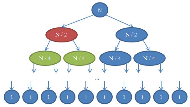
Take a look at the Figure to understand this recursion.

Let's see what's going on here. Each circle represents a call to the mergeSort function. The number written in the circle indicates the size of the array that is being sorted. The top blue circle is the original call to mergeSort, where we get to sort an array of size n. The arrows indicate recursive calls made between functions. The original call to mergeSort makes two calls to mergeSort on two arrays, each of size n / 2. This is indicated by the two arrows at the top. In turn, each of these calls makes two calls of its own to mergeSort two arrays of size n / 4 each, and so forth until we arrive at arrays of size 1. This diagram is called a recursion tree, because it illustrates how the recursion behaves and looks like a tree (the root is at the top and the leaves are at the bottom, so in reality it looks like an inversed tree).
Notice that at each row in the above diagram, the total number of elements is n. To see this, take a look at each row individually. The first row contains only one call to mergeSort with an array of size n, so the total number of elements is n. The second row has two calls to mergeSort each of size n / 2. But n / 2 + n / 2 = n and so again in this row the total number of elements is n. In the third row, we have 4 calls each of which is applied on an n / 4-sized array, yielding a total number of elements equal to n / 4 + n / 4 + n / 4 + n / 4 = 4n / 4 = n. So again we get n elements. Now notice that at each row in this diagram the caller will have to perform a merge operation on the elements returned by the callees. For example, the circle indicated with red color has to sort n / 2 elements. To do this, it splits the n / 2-sized array into two n / 4-sized arrays, calls mergeSort recursively to sort those (these calls are the circles indicated with green color), then merges them together. This merge operation requires to merge n / 2 elements. At each row in our tree, the total number of elements merged is n. In the row that we just explored, our function merges n / 2 elements and the function on its right (which is in blue color) also has to merge n / 2 elements of its own. That yields n elements in total that need to be merged for the row we're looking at.
By this argument, the complexity for each row is Θ( n ). We know that the number of rows in this diagram, also called the depth of the recursion tree, will be log( n ). The reasoning for this is exactly the same as the one we used when analyzing the complexity of binary search. We have log( n ) rows and each of them is Θ( n ), therefore the complexity of mergeSort is Θ( n * log( n ) ). This is much better than Θ( n² ) which is what selection sort gave us (remember that log( n ) is much smaller than n, and so n * log( n ) is much smaller than n * n = n²). If this sounds complicated to you, don't worry: It's not easy the first time you see it. Revisit this section and reread about the arguments here after you implement mergesort in your favourite programming language and validate that it works.
As you saw in this last example, complexity analysis allows us to compare algorithms to see which one is better. Under these circumstances, we can now be pretty certain that merge sort will outperform selection sort for large arrays. This conclusion would be hard to draw if we didn't have the theoretical background of algorithm analysis that we developed. In practice, indeed sorting algorithms of running time Θ( n * log( n ) ) are used. For example, the Linux kernel uses a sorting algorithm called heapsort, which has the same running time as mergesort which we explored here, namely Θ( n log( n ) ) and so is optimal. Notice that we have not proven that these sorting algorithms are optimal. Doing this requires a slightly more involved mathematical argument, but rest assured that they can't get any better from a complexity point of view.

The Learning-to-Program Path

Source

I’ve found my experience to follow that line closely, and came up with this Recursive Recipe for Learning to Program:

1. Follow a tutorial step-by-step even if you don’t always understand what you’re doing. I like to think of Hunter S. Thompson copying the books of the Great Masters on his typewriter. You’re getting a feel for how things are done in your new language/framework. This part should be easy, if boring, because you’re just doing what you’re told. [Incline of Optimism]
2. Rebuild the thing you just made or a slight variation of it. Try not to use the tutorial too much. Realize just how little you understood of what you were doing. [Fear tugs, slowing your ascent]
3. Try to build something simple that you actually want to make. Discover that you have absolutely no idea what you’re doing. [Sea of Despair]
4. Find a new tutorial related to your new project. (Hopefully your tutorials are providing you with increasing background on the language.) Follow the steps. [Slight sense of understanding, rise in self-worth]
5. Rebuild the thing yourself. [Fear]
6. Start a new project. [Despair]
7. Repeat steps 1 through 6.